12.4 STK Astrogator Features

Lambert and cislunar and RPO, oh my! But, not the Dorothy “oh my,” more of the George Takei “oh my.” Complete with a wink. Because everything space is better with Captain Sulu and STK 12.4.

Fast Lambert Profiles

So, let’s start with Lambert. Long-time Astrogator fans may be asking, “Lambert – isn’t that the oldest problem in the book?”

To which we’d respond, “Most astrodynamics books say it’s like the second oldest problem.” So, we’re in good shape.

You may then ask, “Yes, but why only now in STK 12.4? Also, I thought I heard about some Lambert thing back in STK 11.6.”

And, then we’d respond, “Sure, we got started with Lambert for STK 11.6, but now it’s different, nay better!”

In contrast to the Lambert design tool introduced in STK 11.6 — that merely produced Lambert solutions for Astrogator to ingest —, the Lambert options in STK 12. are integrated into Astrogator target sequences as profiles; two profiles, to be specific. The first profile is a simple Lambert solver; you tell it where you want to go with a few options and it gives you the Lambert maneuver(s). Then, you can correct the Lambert arc into the higher-fidelity model with a differential corrector. The second profile is a Lambert search profile. It does some work (in parallel even) to find the best Lambert arc, subject to some constraints.

Again, you ask, “Why not before?”

Well, before we wanted to make Astrogator hard to use — rocket scientists only! In retrospect, that wasn’t the best idea. So, we decided to make it easy. Well, easier. It still is rocket science after all.

Let’s Lambert already!

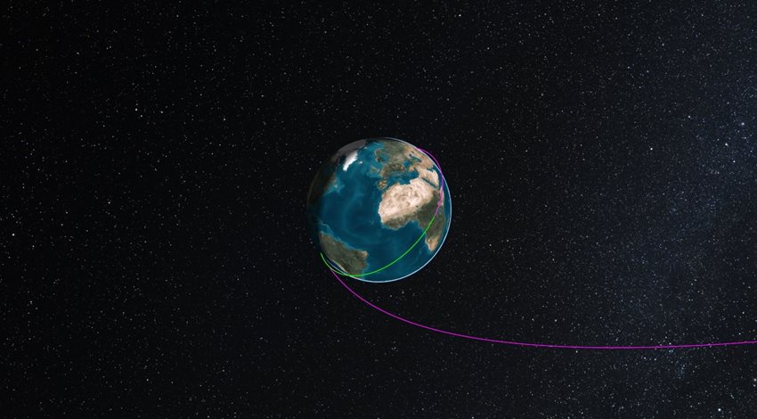
Check it out, there’s a low-Earth orbit in green propagated in Astrogator. Then, a Lambert search profile is employed to find the best departure time — the magenta overlapping the green LEO path — as well as the best arrival time… somewhere. Can you stand the suspense?

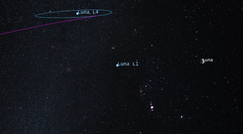
There’s our Lambert arc arriving at the vicinity of the L4 libration point in the Earth–Luna system. Luna is our idealized “three-body” Moon. Check out this tutorial if that last bit made you say, “What?!”. In fact, we inserted into an L4 libration point orbit. Nifty! Note: we surreptitiously changed the view on you from an inertial view in the first image to a rotating frame view in the second. We also didn’t find the absolute best transfer, for our purposes here we went with quick and dirty. Within minutes we had a Lambert transfer to the L4 orbit.

State Transition Matrix

Speaking of that L4 orbit, you’re now probably saying to yourself, “What the heck are the stability characteristics of that orbit? I sure wish I could compute the state transition matrix (STM) after one revolution of that orbit, you know the monodromy matrix. I hear its eigenvalues and eigenvectors will tell me what the linear stability of the orbit is.

No? You’re not saying that to yourself? Well, why not? Let’s do it anyway, you know, for fun.

There are a few caveats: your propagator has to include the STM propagation function and you need to set your report frame to segment appropriately. Then, you can simply run a segment summary report to get the much-desired stability information for your orbit.

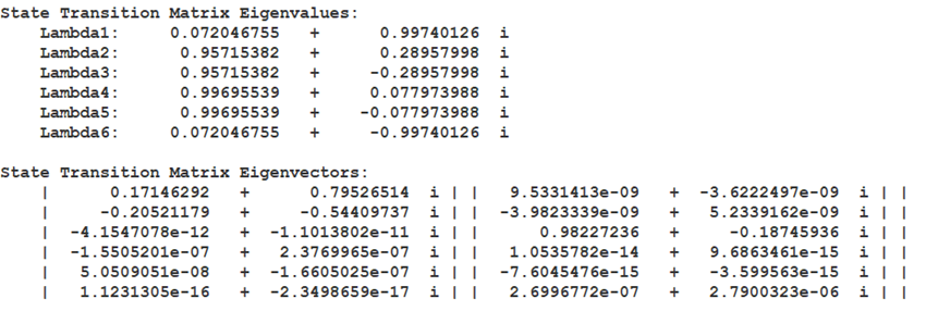
Only the first two of six eigenvectors are shown toward the bottom. This L4 short period orbit is characteristic of four purely complex eigenvalues and two that are very close to one, indicating only a center subspace, i.e., gently perturbed trajectories will somewhat tend to stick around. Of course, the ability to compute and report the STM along with its eigenvalues and eigenvectors is not new for 12.4 — it came in 12.2 —, but we wanted to tell you about it anyway. What is new is the ability to reinitialize the STM from the advanced propagator settings on propagate segments and finite maneuvers. Oh, and you can propagate the STM through finite maneuvers now, too!

The stability information gives us hints into the localized linear motion that can be extended to the underlying nonlinear solutions. From there we can find natural relative motion near our libration point orbits. Relative motion — as in cislunar rendezvous and proximity operations (RPO) — are now nearly possible out-of-the-box (some assembly required, for now). And with that magic initialism, RPO, our journey is mostly complete.

Rendezvous and Proximity Operations (RPO)

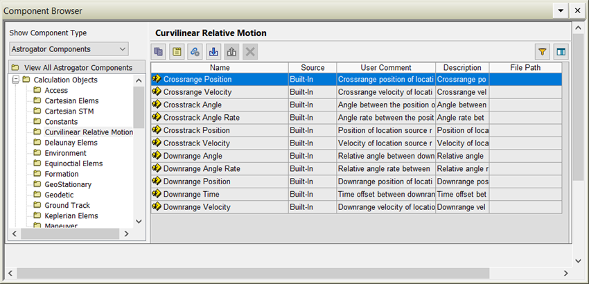
We’ll leave you, dear reader, warm in the assurance of new RPO supporting calculation objects harnessing curvilinear geometry for their underlying computations. These calculation objects are found in the component browser and you can use them everywhere that calculation objects are typically used. They make certain computations more accurate and help speed up convergence. Here they are:

For more information about the new STK 12.4 features, visit agi.com/newstk.

If you take nothing else away from this blog post, it should be, “Oh my.”