Batch vs. Sequential estimation methods in Orbit Determination
- Apr 30, 2018
- Article
- Space Operations
-
 Orbit Determination Tool Kit (ODTK)
Orbit determination is the process, or a set of techniques, for obtaining knowledge about the motion of objects such as moons, planets, and spacecraft relative to the center of mass of the Earth for a specific coordinate system.
Generally speaking, we can say that at least six independent measurements are required to uniquely determine an orbit without a priori knowledge (since a Keplerian orbit is fully characterized by six orbital parameters). For the satellite orbit determination problem, the minimal set of parameters are the position and velocity vectors at a given epoch. This minimal set can be expanded to not just determine the satellite’s orbit, but also to include dynamic and measurement model parameters (such as tracking equipment biases and environmental forces affecting satellite motion), which may be needed to improve the prediction accuracy. The problem of determining the best estimate of the state over time of a spacecraft from observations influenced by random and systematic errors using an approximated mathematical model is referred to as the problem of state estimation.
There are two commonly used approaches for performing OD:
- The batch Least Squares approach where all the data for a fixed period is collected and processed together.
- The Sequential Processing approach, which sequentially updates the state vector to produce a better estimate at each epoch using process noise information.
The batch Least Squares approach is commonly employed for off-line processing of trajectories from LEO spacecraft as the tracking data is typically downloaded once per revolution. On the other hand, in applications involving on-board navigation of spacecraft in real time, the Sequencing Processing (using Kalman filter) is typically used for estimation algorithm.
ODTK (AGI’s Orbit Determination Tool Kit) provides both methods in the same environment. So, what are the differences between the two?
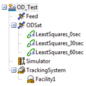
The Least Squares object
From the hierarchical point of view, it is the children of the satellite object:
Pros and cons of both methods
I am now going to summarize the pros and cons of both methods, letting you decide which one best fits your mission needs and requirements.
You can insert as many LS objects as you need (each of them having different characteristics) for result comparison purposes.
For each LS object, you can insert one or more “stages” that define the fit span for that particular run. Each stage is fully configurable, so the results relevant to different runs can be compared. The LS process can also be used to estimate the Ballistic Coefficient and the Solar Radiation Parameter, even if the estimated value is constant over the entire fit span in this case:
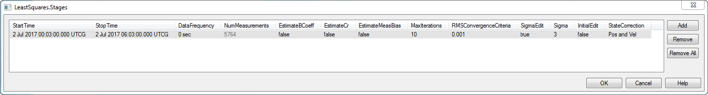
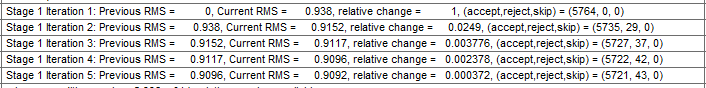
Because the problem is non-linear, an iterative LS method is used until the RMS (Root Mean Square) value between two consecutive runs produces a relative change that is smaller than the convergence threshold.
The Filter object
The sequential processing operated by the filter can be thought as a recursive formulation of the LS method when the whole set of observations is partitioned into statistically independent batches composed by a single measurement. For each measurement, the Kalman filter iterates across two phases:
- The prediction phase implements equations that describe the physical model of our system: from the current state (and its uncertainty), you can then predict which will be the next one (and the relevant uncertainty)
- The correction phase uses the new measurement (relevant to the predicted epoch state) and applies the needed correction according to the confidence level you have (measurement uncertainty)
The Filter is a standalone object in ODTK. Its proprieties allow you to select which satellite, tracking station and tracking data type to consider during the run. It can solve any unknown parameter in the system (e.g., tracking station location or clock biases), with a time-varying estimation. The Filter can also output data to the Smoother, another sequential filter that runs backwards in time to refine the OD solution and perform some consistency checks on the solution found.
| Pros to using batch least squares | Cons to using batch least squares |
| Easy to use | Poor performance with maneuvers |
| Fewer inputs to set | Difficult to find an optimal “fit span” |
| Lots of experienced analysts | Covariance is too optimistic |
| Inverse fails if state is not completely observable | |
| Does not handle dynamic parameters |
| Pros to using a filter | Cons to using a filter |
| Really good performance with maneuvers | Requires a reasonable starting state |
| Realistic error covariance | Fewer experienced analysts |
| Eliminates concept of “fit span” | |
| Adapts & compensates for force model errors |
Author

Orbit Determination Tool Kit (ODTK)
Process tracking data and generate orbit ephemeris with realistic covariance.